A multiscale Gaussian Reproducing Kernel

In this file we look more closely at the multiscale Gaussian Reproducing Kernel (RK) The multiscale Gaussian RK is build as a sum of Gaussian RK with different sigma. In Metamorphosis, the RK is used to parameterize V the space of acceptable vector fields. In practice, it has a smoothing effect on vector fields. However, Gaussian RK erase the high frequency of the vector fields which prevents the vector fields to match small details in the images. To overcome this issue, we can use a multiscale Gaussian RK, that will keep smoothing properties while keeping some high frequency information. It can be seen as a compromise kernel.

The formal definition is: Let \(\Gamma = { \sigma_1, \sigma_2, \ldots, \sigma_n}\) be a list of standard deviations.

\[\mathrm{kernel}_\Gamma = \sum_{\sigma \in \Gamma} \frac {1}{nk_\sigma} \exp\left(\frac{-x^2}{2 \sigma^2}\right)\]

where \(n\) is the number of elements in \(\Gamma\). if normalised is True, \(k\) is equal to:

\[k_\sigma = \sum_{x \in Omega} \exp\left(\frac{-x^2}{2 \sigma^2}\right)\]

else, \(k\) is equal to 1.

First let’s Import the necessary libraries

import numpy as np

from demeter.constants import DLT_KW_IMAGE
import matplotlib.pyplot as plt
import torch
import demeter.utils.reproducing_kernels as rk
import demeter.utils.torchbox as tb

plt.rcParams['text.usetex'] = False

To use the multi-scale Gaussian RK, we need to choose a list of sigma. The larger the sigma, the more the RK will smooth the vector fields. The smaller the sigma, the more the RK will keep the high frequency information of the vector fields. Feel free to change the sigma_list to see the effect of the RK on next figures

sigma_list = [
        # (1,1),
        (2,2),
        (5,5),
        (10,10),
        # (16,16)
        # (20,20),
    ]
normalize = True

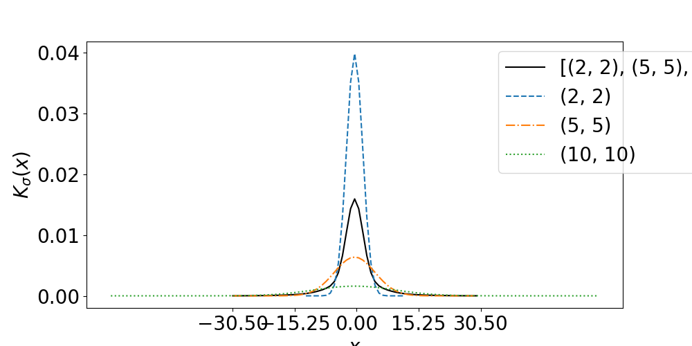
First let’s see the kernels of the Gaussian Reproducing Kernel for different sigma superimposed on the Multi-scale Gaussian Reproducing Kernel. We plot a 1D slice of the 2D kernels at its center.

def see_kernels_filter_2D(sigma_list,ax=None, force_xticks=None):

    mono_gauss = [
        rk.GaussianRKHS(s,'constant',normalized=normalize)
        for s in sigma_list
    ]
    multi_RKHS = rk.Multi_scale_GaussianRKHS(sigma_list, normalized=normalize)
    font_size= 20
    if ax is None:
        fig,ax = plt.subplots(figsize=(10,5))
    kernel_multi = multi_RKHS.kernel
    _,h,w = kernel_multi.shape
    tick_max = w if force_xticks is None else force_xticks
    x_scale = (torch.arange(w) - w/2)
    ax.plot(x_scale,kernel_multi[0,h//2],label=str(sigma_list),c='black')
    style = ['--','-.',':']

    for i,s in enumerate(sigma_list):
        kernel_m = mono_gauss[i].kernel
        _,hh,ww = kernel_m.shape

        # x_scale = (torch.arange(ww)+((tick_max - ww)/2))
        x_scale = (torch.arange(ww) - ww/2)
        ax.plot(x_scale,
                mono_gauss[i].kernel[0,hh//2],
                label=str(s),linestyle=style[i - 3*(i//3)])
    ax.set_ylabel(r'$K_\sigma(x)$',fontsize=font_size)
    ax.set_xlabel(r'$x$',fontsize=font_size)
    # tick_max = w if force_xticks is None else force_xticks
    x_ticks = np.linspace(-tick_max/2,tick_max/2,5)
    ax.set_xticks(x_ticks)
    ax.tick_params(axis='both',
                   #which='minor',
                   labelsize=font_size)
    ax.legend(loc='upper left',
              fontsize=font_size,
              bbox_to_anchor=(.75, 1.),
              # ncol=len(sigma_list)+1
              )

see_kernels_filter_2D(sigma_list)

Now let’s visualize the convolution of an image by the Gaussian RKs and the multi-scale Gaussian RK. For visualization purposes, we will use images but keep in mind that the RK is intended to be used on vector fields.

def see_im_convoled_by_kernel(kernelOp,I,ax):
    _,_,H,W = I.shape
    if kernelOp is None:
        I_g =I
    else:
        I_g = kernelOp(I)
    ax[0].imshow(I_g[0,0], **DLT_KW_IMAGE)
    ax[1].plot(I_g[0,0,H//2])

def see_mono_kernels(I,sigma_list):
    fig,ax = plt.subplots(2,len(sigma_list)+2,figsize=(20,5))
    fig.suptitle(f'Convolution of an image by a reproducing kernel, {sigma_list}')
    see_im_convoled_by_kernel(None,I,ax[:,0])
    for i,s in enumerate(sigma_list):
        grk = rk.GaussianRKHS(s,'constant')
        see_im_convoled_by_kernel(grk,I,ax[:,i+1])
        ax[0,i+1].set_title(r'$\sigma = $'+str(grk.sigma))
    mgrk = rk.Multi_scale_GaussianRKHS(sigma_list, normalized=normalize)
    see_im_convoled_by_kernel(mgrk,I,ax[:,-1])
    ax[0,-1].set_title(r"Multi-scale ")

# You can choose different images to see the effect of the RK on them
img_name = '01'           # simple disk
img_name = 'sri24'      # slice of a brain
img = tb.reg_open(img_name,size = (300,300))


see_mono_kernels(img,sigma_list)

plt.show()